The performance of the Revolution or any magnetic compass depends on how well its parameters are adjusted for the operating environment. Accuracy, repeatability, speed of response, rejection of anomalous measurements, and power consumption can be optimized by careful tuning of coefficients that adapt the compass to different conditions. For example, in a hand-held surveying application, low power consumption and high accuracy are important for intermittent samples. Operating in SAMPLE mode would be appropriate, and automatically entering sleep mode between samples would minimize power consumption. Parameters used only in RUN mode can be ignored. These include settings for magnetic and tilt filters; settings for the magnetic alarm; and settings for the non-linear heading filter.
In contrast, automatic antenna positioning requires continuous measurements in the presence of mechanical noise and magnetic anomalies. The RUN mode of operation is required, and settings for filters and alarms must be adjusted to account for operating conditions. If fast, large-angle movements are to be ignored, the non-linear heading filter can be enabled. If vibration from engine noise, ocean waves, or nearby heavy equipment causes liquid tilt sensor oscillation, the rate gyros (Revolution GS only) should be enabled and the complementary filter time constant is set to optimize tilt angle estimation.
For all applications, the compass accuracy should be verified in-situ by performing a magnetic calibration. This entails first capturing a vertical reference in a nearby location free of magnetic interference, then taking measurements about a circle with the compass mounted in place. The vertical reference can be skipped if you are convinced that there is no vertical component of hard iron.
Factors Affecting Accuracy
There are a number of factors that can potentially affect the accuracy and repeatability of the compass. The following list explains the mechanism of each factor and presents an order of magnitude of its effect on accuracy.
Static Permanent Magnetism
The source of a local permanent magnetic field can be a piece of hard iron (hence the common name), a constant DC current, or some other type of magnet. This source of error can be significantly reduced by calibration. The curve in Figure 1 shows that a residual error of 0.1% of the earth’s magnetic field on both X and Y axes produces a peak accuracy error of 0.20° at 66° inclination (middle US).
The error varies sinusoidally with direction and produces a single cycle for each rotation of the compass. Phase depends on the signs and magnitudes of errors on each axis. The magnitude of the error depends on magnetic inclination because the residual hard iron error is expressed as a fraction of the total field strength.
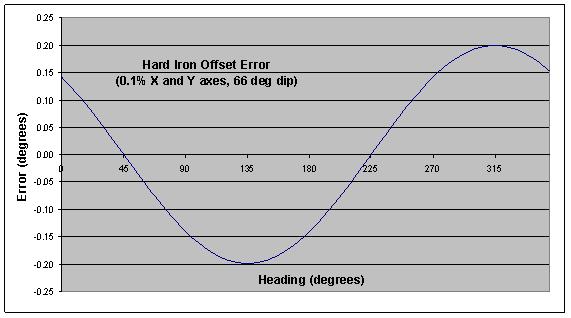
Figure 1 – Hard Iron Heading Error
Fortunately, a residual Z-axis error is less critical. This error comes into play only when the compass card is tilted from level. At 30° tilt, a Z-axis error of 0.3% would be required to produce the same 0.2° peak accuracy error at 66° dip. The accuracy error decreases with decreasing tilt.
This is fortunate because it can be difficult to determine the Z-axis hard iron coefficient. When the compass is mounted in a large vehicle, it is impractical to turn the vehicle over in order to get good calibration data. An estimate of the Z coefficient can be made as long as some tilted data is collected, but a reasonable estimate may still require tilt angles that can’t be achieved.
To eliminate this problem, the Revolution allows an optional two-step Z-axis calibration. Reference data is first collected outside the vehicle, in an area free of magnetic interference. When the compass is mounted in the vehicle, the measured vertical component is compared to the reference data to calculate the coefficient. As long as the compass is within a few degrees of level during both measurements, the calculated result is accurate.
Static Induced Magnetism
When you bring a magnet in contact with a metal paper clip the paper clip becomes magnetized. When the magnet and paper clip are separated, the paper clip no longer retains its temporary, or induced, magnetism. Soft iron, alloys of iron and nickel, common steel, and some types of stainless steel can all be easily magnetized, even in a weak field.
When these materials are in the vicinity of the compass and rotate with the compass, they become magnetized and demagnetized depending on their orientation to the earth’s magnetic field. Instead of seeing a constant field that would produce a perfect circle as the compass turns, the compass sees a field of varying magnitude that maps an elliptical shape. This induced magnetism gives rise to a heading accuracy error as shown in the example of Figure 2.
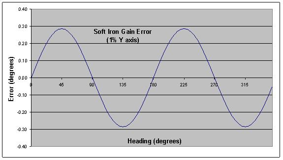
Figure 2 – Soft Iron Heading Error
When the compass is rotated in a level plane, the error varies sinusoidally and produces two cycles per revolution of the compass. In the figure, peaks are located at 45°, 135°, 225°, and 315° because the gain error is aligned with an axis, and there are no hard-iron errors (so the errors at 0, 90, 180 and 270 are zero). In real world applications, the ellipse axis could be aligned at any angle.
In three dimensions, the locus of points would map to an ellipsoid instead of a perfect sphere. In this case, a 3×3 matrix of gain coefficients is needed to compensate. A minimum of 12 independent measurements is needed to determine 9 soft-iron gains and 3 hard-iron offsets.
If the compass is only being used near level, then a simpler, two-dimensional compensation may be adequate. The Revolution PC software includes an algorithm to estimate 2D soft-iron coefficients based on the approach set forth in “Direct Least Squares Fitting of Ellipses,” by Fitzgibbon et al. in IEEE Transactions on Pattern Analysis and Machine Intelligence, Vol. 21, No. 5, May, 1999. The software reports the ellipticity, in percent, of the ellipse that best fits the collected data. This metric can be used to decide if soft-iron compensation is needed.
In situations where soft-iron is significant, it may be better to relocate the compass. First, a two-dimensional compensation is only approximate, and small variations in tilt may produce dramatic changes in the soft-iron ellipse. Proper compensation may require that three-dimensional data be collected and analyzed to produce the full 3×3 gain matrix.
Second, soft magnetic materials that give rise to induced magnetism also exhibit varying degrees of remanence, the tendency to remain magnetized after a magnetizing force is removed. The magnetization of the material may change over time due to exposure to vibration, temperature changes, and varying electrical and magnetic fields. This results in hard-iron errors that must be periodically compensated to maintain accuracy.
If there is no alternative and 3D soft iron must be compensated, the Revolution PC program provides an option to collect 3D data and calculate the optimum 12 compensation coefficients. The iterative algorithm works to find the ellipsoid that best fits the collected data by minimizing the sum of the squared geometric distances between the collected data and the parametric ellipsoid.
Time Varying Magnetic Fields
A time varying magnetic field in the vicinity of the compass cannot be compensated. Its frequency must be above the pass band of the compass (i.e. greater than 30 Hz), or it must be eliminated. The Revolution’s measurement cycle rate of 27.5 Hz is chosen to maximize attenuation of 50 Hz to 60 Hz signals associated with AC power systems.
To estimate the order of magnitude effect of a DC current near the compass magnetometer, use Ampere’s law to calculate the magnetic field near a long wire: , where Gauss-meter / amp.
A long wire carrying 25 mA of current located 50 mm from the magnetometer produces a 1 mG (100 nT) magnetic disturbance at the sensor. In the middle of the US, where inclination (dip angle) is roughly 66°and the earth’s magnetic field strength is about 500 mG, this can result in a 0.3°heading error.
Tilt Measurement Errors
Errors in pitch and roll measurements give rise to single-cycle heading errors that cannot be differentiated from heading error caused by residual hard-iron. The plot in Figure 3 shows how an error as small as 0.1° on both X and Y axes affects heading accuracy at 66° magnetic inclination (dip angle). The phase of this curve depends on the relative signs and magnitudes of the separate X-axis and Y-axis errors.
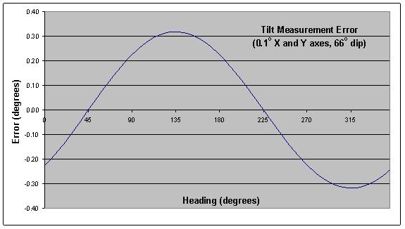
Figure 3 – Effect of Tilt Error on Heading Accuracy
Compare the shape and phase of the curve in Figure 3 to the hard-iron error curve in Figure 1. In this case, the curves are not in phase, and the two sources of error tend to cancel each other. The resulting peak error is reduced by a factor of three as shown in the curve labeled “Errors Cancel” in Figure 4. But change the signs on both pitch and roll errors, and the two curves align in phase, producing the “Errors Reinforce” result also shown in Figure 4.
Tilt measurement errors can be caused by one or more of the following:
1. sensor offset and/or gain errors
2. sensor cross-axis coupling
3. misalignment of tilt and magnetic sensor axes
4. uncompensated horizontal acceleration
5. poor sensor quality
In applications where the compass cannot be held perfectly steady, the error due to horizontal acceleration can be pronounced. Although the rate gyros (Revolution GS) will initially compensate, if the acceleration persists, it will eventually affect the measurement. For a modest constant horizontal acceleration of 0.05g (roughly 1 mile per hour per second), the tilt measurement error is 2.9° (obtained by calculating
tan-10.05). For the example 66° magnetic inclination used above, the result is a sinusoidal heading error of 6.5° peak magnitude.
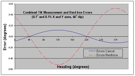
Figure 4 – Combined Effect of Hard Iron and Tilt Errors
Magnetic Inclination (Dip Angle)
Near its magnetic poles, the overall strength of the earth’s magnetic field increases. But the horizontal component decreases substantially, making navigation by magnetic compass nearly impossible. For mechanical compasses, the needle dips excessively, trying to align with almost vertical lines of force. For an electronic compass, accuracy decreases because the horizontal field is smaller and because the effect of tilt errors is more pronounced.
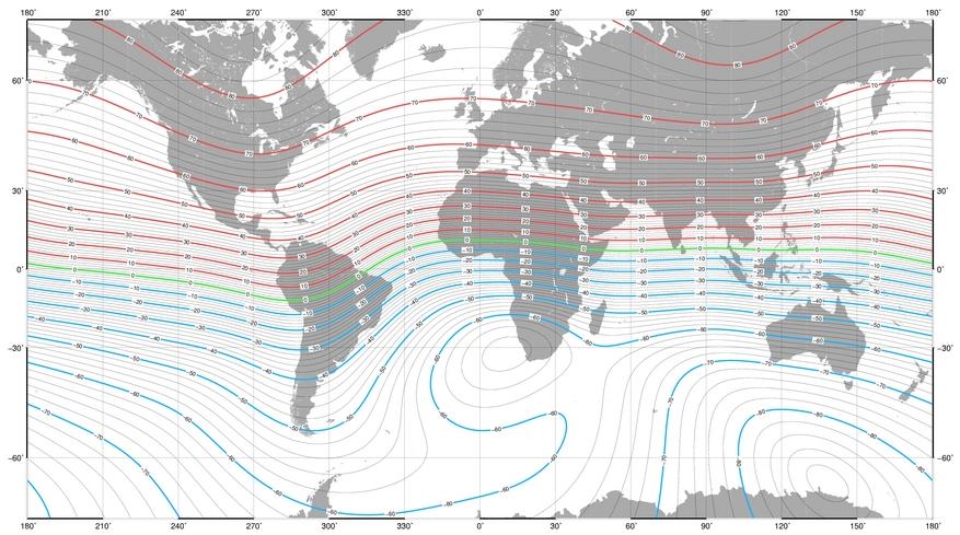
Figure 5 – Magnetic Inclination Contour Lines (in degrees)
The map in Figure 5 shows lines of constant dip angle around the globe. Each of the lines is separated by 2°. The map is based on the US/UK world magnetic model for the year 2005.
Near the magnetic equator, tilt measurement errors have very little influence on compass heading. Between ±5° dip, a 1° error in tilt produces no greater than 0.09° heading error. In northern Alaska (80° dip), the same 1° tilt error results in as much as 6° heading error.
Summary
If you have any questions about optimizing compass performance, for True North’s products or other manufacturers, please do not hesitate to contact us.
Receive A Free Quote